Introduction
Version 2.0 of the synthdid package introduces a modern
formula-based interface similar to lm(),
plm(), and glm(). This vignette demonstrates
how to use the new interface while maintaining full backward
compatibility with existing code.
Why a New Interface?
The new formula interface offers several advantages:
- More intuitive: Follows standard R modeling conventions
- Less code: Single function call instead of multiple steps
-
Better integration: Works with standard R tools
(
summary(),coef(),confint()) -
Easier comparison: Switch between estimators with
update() - Self-documenting: Formula syntax is clearer than matrix indexing
Backward Compatibility
All existing code continues to work! The original matrix-based interface is fully supported:
# Old interface (still works)
data("california_prop99")
setup <- panel.matrices(california_prop99)
old_result <- synthdid_estimate(setup$Y, setup$N0, setup$T0)
old_result
#> synthdid: -15.604 +- NA. Effective N0/N0 = 16.4/38~0.4. Effective T0/T0 = 2.8/19~0.1. N1,T1 = 1,12. [NOT CONVERGED]
Basic Usage
Simple Estimation
The new interface uses a formula to specify the outcome and treatment variables:
# New formula interface
result <- synthdid(PacksPerCapita ~ treated,
                   data = california_prop99,
                   index = c("State", "Year"))
result
#> Synthetic Difference-in-Differences Estimate
#>
#> Call:
#> synthdid(formula = PacksPerCapita ~ treated, data = california_prop99,
#>     index = c("State", "Year"))
#>
#> Treatment Effect:  -15.6
#>
#> Units:        38 control, 1 treated
#> Time Periods: 19 pre-treatment, 12 post-treatment
#>
#> Convergence:  NOT CONVERGED - lambda (10000/10000 iters), omega (10000/10000 iters)
#>               Consider increasing max.iter. Use summary() for details.
The formula PacksPerCapita ~ treated specifies: -
Left side: Outcome variable
(PacksPerCapita) - Right side: Treatment
indicator (treated)
The index argument specifies the panel structure: -
First element: Unit identifier (State) - Second element:
Time identifier (Year)
Standard R Methods
The new interface returns objects that work with standard R functions:
# Extract treatment effect
coef(result)
#>   treated
#> -15.60379

# Get confidence intervals (requires SE computation)
# confint(result)  # Would compute SE automatically

# Summary statistics
summary(result, fast = TRUE)  # Use fast=TRUE for jackknife SE
#> Call:
#> synthdid(formula = PacksPerCapita ~ treated, data = california_prop99,
#>     index = c("State", "Year"))
#>
#> Treatment Effect Estimate:
#>         Estimate
#> treated    -15.6 NA NA NA
#>
#> Dimensions:
#>                          Value
#>  Treated units:           1.000
#>  Control units:          38.000
#>  Effective controls:     16.388
#>  Post-treatment periods: 12.000
#>  Pre-treatment periods:  19.000
#>  Effective periods:       2.784
#>
#> Top Control Units (omega weights):
#>               Weight
#> Nevada         0.124
#> New Hampshire  0.105
#> Connecticut    0.078
#> Delaware       0.070
#> Colorado       0.058
#>
#> Top Time Periods (lambda weights):
#>      Weight
#> 1988  0.427
#> 1986  0.366
#> 1987  0.206
#>
#> Convergence Status:
#>   Overall: NOT CONVERGED
#>   Lambda:  ✗ (10000/10000 iterations, 100.0% utilization)
#>   Omega:   ✗ (10000/10000 iterations, 100.0% utilization)
#>
#>   Recommendation: Consider increasing max.iter or relaxing min.decrease.
#>   Use synthdid_convergence_info() for detailed diagnostics.
Comparing Estimators
One of the most powerful features is the ability to easily compare different panel data estimators.
Method Selection
You can choose the estimator at estimation time:
# Synthetic Difference-in-Differences (default)
synthdid_est <- synthdid(PacksPerCapita ~ treated,
                         data = california_prop99,
                         index = c("State", "Year"),
                         method = "synthdid")

# Pure Difference-in-Differences
did_est <- synthdid(PacksPerCapita ~ treated,
                    data = california_prop99,
                    index = c("State", "Year"),
                    method = "did")

# Synthetic Control
sc_est <- synthdid(PacksPerCapita ~ treated,
                   data = california_prop99,
                   index = c("State", "Year"),
                   method = "sc")
Updating Models
The update() function allows you to modify an existing
model:
Side-by-Side Comparison
# Compare all three estimators
comparison <- data.frame(
  Method = c("SynthDID", "DID", "SC"),
  Estimate = c(coef(synthdid_est), coef(did_est), coef(sc_est))
)
print(comparison)
#>     Method  Estimate
#> 1 SynthDID -15.60379
#> 2      DID -27.34911
#> 3       SC -19.61966
The estimates differ because each method makes different assumptions: - SynthDID: Weights both units and time periods - DID: Equal weights on all control units and time periods - SC: Weights only control units (equal time weights)
Standard Errors
Computing Standard Errors
You can request standard errors at estimation time:
# Bootstrap SE (most reliable, but slow)
result_boot <- synthdid(PacksPerCapita ~ treated,
                        data = california_prop99,
                        index = c("State", "Year"),
                        se = TRUE,
                        se_method = "bootstrap",
                        se_replications = 200)

# Jackknife SE (faster)
result_jack <- synthdid(PacksPerCapita ~ treated,
                        data = california_prop99,
                        index = c("State", "Year"),
                        se = TRUE,
                        se_method = "jackknife")

# Placebo SE (for single treated unit)
result_placebo <- synthdid(PacksPerCapita ~ treated,
                           data = california_prop99,
                           index = c("State", "Year"),
                           se = TRUE,
                           se_method = "placebo",
se_replications = 100)Parallel Processing
For faster SE computation with bootstrap or placebo methods, use parallel processing:
library(future)

# Set up parallel processing
plan(multisession, workers = 4)

# Estimate with parallel SE computation
result <- synthdid(PacksPerCapita ~ treated,
                   data = california_prop99,
                   index = c("State", "Year"),
                   se = TRUE,
                   se_method = "bootstrap",
                   se_replications = 200)

# Reset to sequential
plan(sequential)
For a comprehensive guide on parallel processing,
including performance comparisons, best practices, and when to use
sequential vs parallel, see
vignette("parallel-processing").
Thread Management
The package automatically manages BLAS threads to prevent thread oversubscription when using parallel workers. Without proper management:
- Bad scenario: 4 parallel workers × 8 BLAS threads = 32 threads on a 4-core machine
- Performance: Severe degradation due to context switching
The package automatically: 1. Detects when parallel processing is active 2. Sets BLAS to single-threaded mode for each worker 3. Restores BLAS threads after completion
Result: 4 parallel workers × 1 BLAS thread = 4 threads (optimal for 4 cores)
For best thread control, install the optional
RhpcBLASctl package:
install.packages("RhpcBLASctl")This provides reliable control over OpenBLAS and MKL thread counts. Without it, the package falls back to environment variables which may require an R restart to take effect.
Predictions and Diagnostics
Treatment Effect by Period
The predict() function extracts the treatment effect for
each post-treatment period:
# Effect curve
effect_curve <- predict(result, type = "effect")
print(effect_curve)
#>  [1]  -4.844930  -4.325765  -8.653504  -8.419076 -12.545421 -16.106184
#>  [7] -18.905726 -19.350095 -20.883473 -22.781531 -25.944883 -24.484840
# Plot effect curve
plot(effect_curve, type = "b",
     xlab = "Post-Treatment Period",
     ylab = "Treatment Effect",
     main = "Treatment Effect Over Time")
abline(h = 0, lty = 2, col = "gray")
Counterfactual Predictions
What would have happened to California without Prop 99?
# Counterfactual outcomes for treated units
counterfactual <- predict(result, type = "counterfactual")

# Show first 5 periods
counterfactual[, 1:5]
#>     1970     1971     1972     1973     1974
#> 141.8860 145.2028 149.8275 149.1232 150.1937
Actual Treated Outcomes
# Actual observed outcomes for treated units
treated_outcomes <- predict(result, type = "treated")

# Show first 5 periods
treated_outcomes[, 1:5]
#>  1970  1971  1972  1973  1974
#> 123.0 121.0 123.5 124.4 126.7
Residuals
Extract residuals from different parts of the model:
# Control unit residuals
resid_control <- residuals(result, type = "control")
cat("Control residuals dimension:", dim(resid_control), "\n")
#> Control residuals dimension: 38 31
cat("Mean absolute residual:", mean(abs(resid_control)), "\n")
#> Mean absolute residual: 22.72082

# Pre-treatment period residuals
resid_pretreat <- residuals(result, type = "pretreatment")
cat("Pre-treatment residuals dimension:", dim(resid_pretreat), "\n")
#> Pre-treatment residuals dimension: 39 19

# All residuals
resid_all <- residuals(result, type = "all")
cat("All residuals dimension:", dim(resid_all), "\n")
#> All residuals dimension: 39 31Covariate Adjustment
The formula interface supports time-varying covariates using the
| operator:
# With covariates (if available in your data)
result_cov <- synthdid(PacksPerCapita ~ treated | log_income + unemployment,
                       data = your_data,
                       index = c("State", "Year"))
The formula
outcome ~ treatment | covariate1 + covariate2 specifies: -
Left of ~: Outcome variable - Right of ~, left
of |: Treatment indicator - Right of |:
Covariates to adjust for
Plotting
All existing plotting functions work with the new interface:
# Standard synthdid plot
plot(result)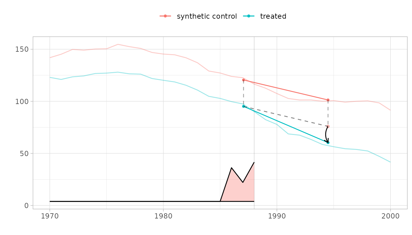
# Control unit contribution plot
synthdid_units_plot(result)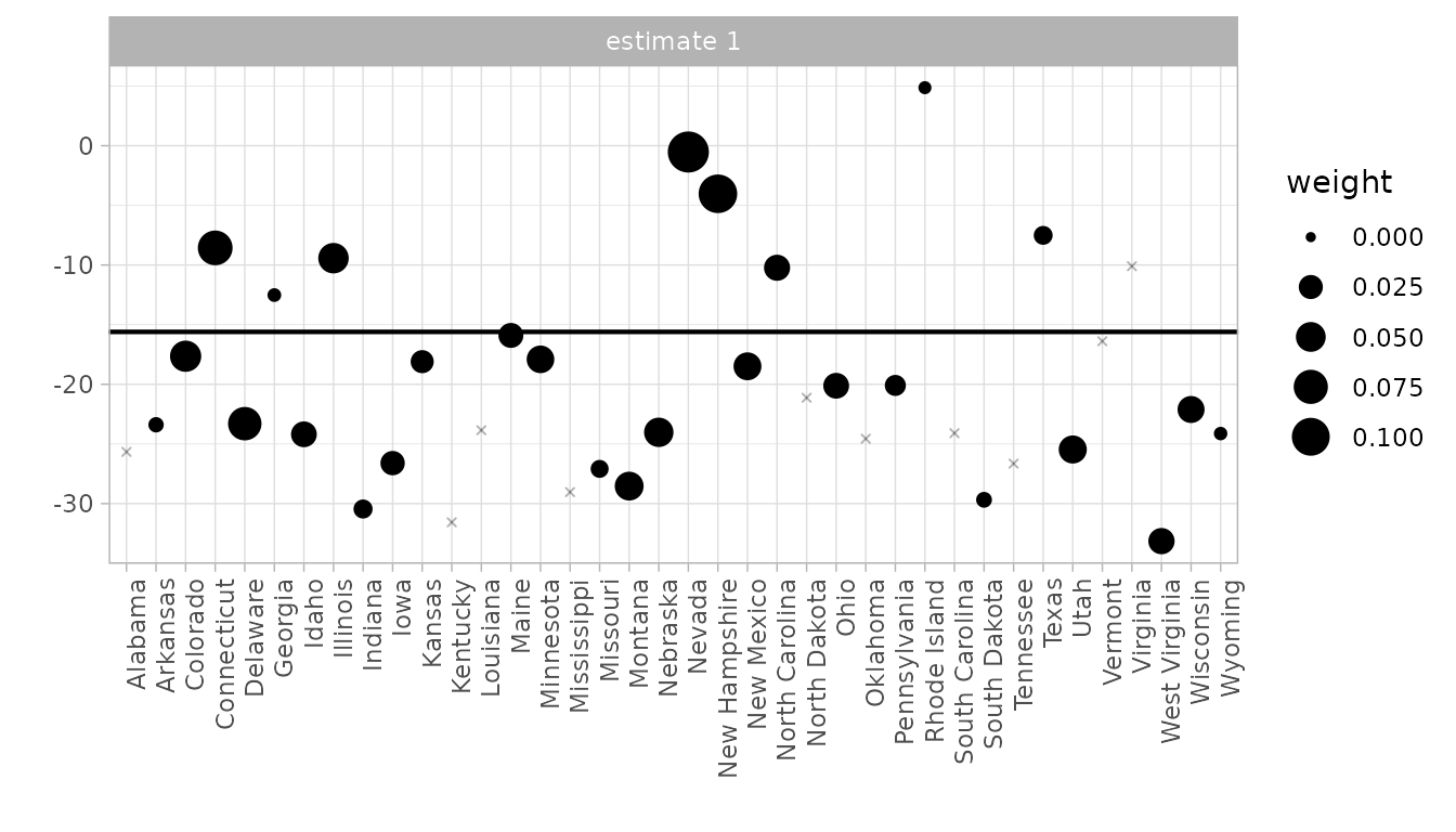
# Check pre-treatment parallel trends
plot(result, overlay = 1)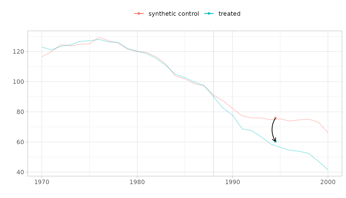
Working with Model Objects
Extracting Components
The new interface creates rich model objects with many components:
# Get the call
attr(result, "call")
#> synthdid(formula = PacksPerCapita ~ treated, data = california_prop99,
#>     index = c("State", "Year"))

# Get the formula
attr(result, "formula")
#> PacksPerCapita ~ treated

# Get panel index
attr(result, "index")
#>    unit    time
#> "State"  "Year"

# Get weights
weights <- attr(result, "weights")
names(weights)
#> [1] "omega"       "lambda"      "lambda.vals" "vals"        "omega.vals"

# Lambda (time weights)
head(weights$lambda)
#>      [,1]
#> [1,]    0
#> [2,]    0
#> [3,]    0
#> [4,]    0
#> [5,]    0
#> [6,]    0

# Omega (unit weights)
head(weights$omega)
#>             [,1]
#> [1,] 0.000000000
#> [2,] 0.003441829
#> [3,] 0.057512787
#> [4,] 0.078287288
#> [5,] 0.070368123
#> [6,] 0.001588411
Model Information
# Data information
data_info <- attr(result, "data_info")
data_info
#> $outcome
#> [1] "PacksPerCapita"
#>
#> $treatment
#> [1] "treated"
#>
#> $covariates
#> character(0)
#>
#> $n_units
#> [1] 39
#>
#> $n_periods
#> [1] 31
Advanced Usage
Custom Options
You can pass any option from synthdid_estimate() to the
formula interface:
Summary
Quick Reference
| Task | Command |
|---|---|
| Basic estimation | synthdid(outcome ~ treatment, data, index) |
| With SE | synthdid(..., se = TRUE, se_method = "bootstrap") |
| With covariates | synthdid(outcome ~ treatment \| cov1 + cov2, ...) |
| Method selection | synthdid(..., method = "synthdid"/"did"/"sc") |
| Extract coefficient | coef(result) |
| Confidence interval | confint(result) |
| Summary | summary(result) |
| Effect curve | predict(result, type = "effect") |
| Counterfactual | predict(result, type = "counterfactual") |
| Residuals | residuals(result, type = "control") |
| Fitted values | fitted(result) |
| Update model | update(result, method = "did") |
| Plot | plot(result) |
Migration from Old Interface
| Old Interface | New Interface |
|---|---|
setup <- panel.matrices(data) |
— |
synthdid_estimate(setup$Y, setup$N0, setup$T0) |
synthdid(outcome ~ treatment, data, index) |
c(result) |
coef(result) |
sqrt(vcov(result)) |
confint(result) (automatic SE) |
| Manual effect curve calculation | predict(result, type = "effect") |
| Custom comparison code | update(result, method = "did") |
Next Steps
- See
vignette("synthdid")for the original introduction - See
vignette("more-plotting")for plotting examples - See
?synthdidfor complete function documentation - See
INTERFACE_IMPROVEMENTS.mdfor implementation details