Getting Started with synthdid

library(synthdid)
library(ggplot2)
library(dplyr)
library(tidyr)
set.seed(12345)

What Is Synthetic Difference-in-Differences?

Panel data—repeated observations of multiple units over time—are the workhorse of causal inference in the social sciences. When some units receive a treatment and others do not, two classical approaches exist for estimating the treatment effect:

Difference-in-Differences (DID) compares the change in outcomes before and after treatment between treated and control units. It assumes that, absent treatment, both groups would have followed parallel trends. DID weights all control units and all pre-treatment periods equally.
Synthetic Control (SC) constructs a weighted average of control units that closely matches the treated unit’s pre-treatment outcome trajectory. It does not assume parallel trends in the same way as DID, but it also does not difference out time effects—the counterfactual must match the treated unit’s level, not just its trend.

Synthetic Difference-in-Differences (SDID), proposed by Arkhangelsky et al. (2021), combines both ideas. It selects:

Unit weights (omega, $\omega$ ): like SC, a weighted average of control units that matches the treated unit’s pre-treatment trajectory.
Time weights (lambda, $\lambda$ ): like DID, but with weights that emphasize pre-treatment periods most relevant for the counterfactual, rather than weighting all periods equally.

This double-weighting typically yields better pre-treatment fit than DID and more robustness than SC. The estimator is implemented in this package via a Frank-Wolfe optimization algorithm.

Data Format

The package expects long-format panel data: one row per unit-period, with columns identifying the unit, the time period, the outcome, and a binary treatment indicator.

data("california_prop99")
head(california_prop99)
#>         State Year PacksPerCapita treated
#> 1     Alabama 1970           89.8       0
#> 2    Arkansas 1970          100.3       0
#> 3    Colorado 1970          124.8       0
#> 4 Connecticut 1970          120.0       0
#> 5    Delaware 1970          155.0       0
#> 6     Georgia 1970          109.9       0

The built-in california_prop99 dataset contains annual cigarette consumption (PacksPerCapita) for US states from 1970 to 2000. California (treated = 1) passed Proposition 99 in 1989, raising the cigarette tax. All other states serve as controls.

Basic Estimation

The `synthdid()` Formula Interface

The primary entry point is synthdid(), which uses a formula interface similar to lm():

result <- synthdid(PacksPerCapita ~ treated,
                   data = california_prop99,
                   index = c("State", "Year"))

The formula PacksPerCapita ~ treated specifies:

Left of ~: the outcome variable.
Right of ~: the binary treatment indicator (0/1).

The index argument identifies the two panel dimensions:

First element: the unit identifier ("State").
Second element: the time identifier ("Year").

The returned object supports standard R generics:

# Point estimate of the average treatment effect
coef(result)
#>   treated 
#> -15.60379

# Full summary (uses jackknife SE by default for speed)
summary(result, fast = TRUE)
#> Call:
#> synthdid(formula = PacksPerCapita ~ treated, data = california_prop99, 
#>     index = c("State", "Year"))
#> 
#> Treatment Effect Estimate:
#>         Estimate         
#> treated    -15.6 NA NA NA
#> 
#> Dimensions:
#>                          Value 
#>  Treated units:           1.000
#>  Control units:          38.000
#>  Effective controls:     16.388
#>  Post-treatment periods: 12.000
#>  Pre-treatment periods:  19.000
#>  Effective periods:       2.784
#> 
#> Top Control Units (omega weights):
#>               Weight
#> Nevada         0.124
#> New Hampshire  0.105
#> Connecticut    0.078
#> Delaware       0.070
#> Colorado       0.058
#> 
#> Top Time Periods (lambda weights):
#>      Weight
#> 1988  0.427
#> 1986  0.366
#> 1987  0.206
#> 
#> Convergence Status:
#>   Overall: NOT CONVERGED
#>   Lambda:  ✗ (10000/10000 iterations, 100.0% utilization)
#>   Omega:   ✗ (10000/10000 iterations, 100.0% utilization)
#> 
#>   Recommendation: Consider increasing max.iter or relaxing min.decrease.
#>   Use synthdid_convergence_info() for detailed diagnostics.

Accessing Weights

The SDID estimate is defined by the weights it selects. You can inspect them directly:

weights <- attr(result, "weights")

# Unit weights: one per control state
head(weights$omega, 10)
#>              [,1]
#>  [1,] 0.000000000
#>  [2,] 0.003441829
#>  [3,] 0.057512787
#>  [4,] 0.078287288
#>  [5,] 0.070368123
#>  [6,] 0.001588411
#>  [7,] 0.031468210
#>  [8,] 0.053387823
#>  [9,] 0.010135485
#> [10,] 0.025938629

# Time weights: one per pre-treatment year
head(weights$lambda, 10)
#>       [,1]
#>  [1,]    0
#>  [2,]    0
#>  [3,]    0
#>  [4,]    0
#>  [5,]    0
#>  [6,]    0
#>  [7,]    0
#>  [8,]    0
#>  [9,]    0
#> [10,]    0

Most omega weights will be zero or near-zero—SDID selects a sparse set of donor units, much like SC. The time weights typically concentrate on periods close to the treatment onset.

The Three Estimators

The method argument controls which estimator is used. All three are special cases of the same underlying framework and share the same interface:

sdid_est <- synthdid(PacksPerCapita ~ treated, data = california_prop99,
                     index = c("State", "Year"), method = "synthdid")

sc_est   <- synthdid(PacksPerCapita ~ treated, data = california_prop99,
                     index = c("State", "Year"), method = "sc")

did_est  <- synthdid(PacksPerCapita ~ treated, data = california_prop99,
                     index = c("State", "Year"), method = "did")

data.frame(
  Method   = c("SDID", "SC", "DID"),
  Estimate = round(c(coef(sdid_est), coef(sc_est), coef(did_est)), 2)
)
#>   Method Estimate
#> 1   SDID   -15.60
#> 2     SC   -19.62
#> 3    DID   -27.35

How They Differ

The three estimators differ in what they fix and what they optimize:

Estimator	Unit weights ( $\omega$ )	Time weights ( $\lambda$ )	Intercept adjustment
DID	Uniform (1/N₀)	Uniform (1/T₀)	Yes
SC	Optimized	All zero	No
SDID	Optimized	Optimized	Yes

DID passes omega = rep(1/N0, N0) and lambda = rep(1/T0, T0) — equal weights on everything. The treatment effect is the simple difference-in-differences.
SC optimizes omega to match the treated unit’s pre-treatment trajectory, but sets all lambda to zero and disables the intercept. The counterfactual must match the treated unit’s level.
SDID optimizes both omega and lambda, and includes an intercept. This allows it to match trends even when levels differ.

You can switch between methods with update() without re-specifying the model:

# Start from SDID, switch to DID
did_from_update <- update(sdid_est, method = "did")
coef(did_from_update)
#>   treated 
#> -27.34911

Visualizing the Differences

The built-in plot() method shows the treated trajectory, the synthetic control, and the estimated treatment effect. Comparing across methods reveals how different weighting strategies produce different counterfactuals:

plot(sdid_est, se.method = "placebo")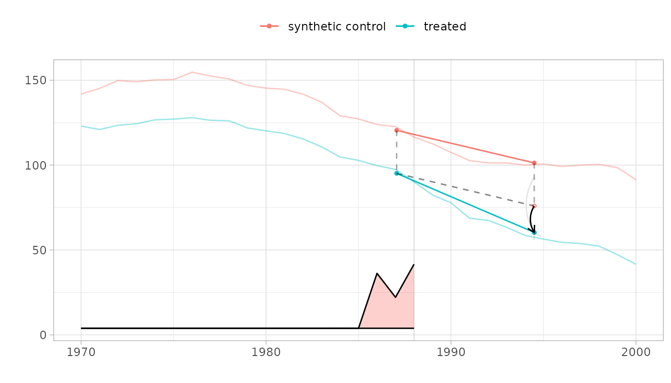

The parallelogram overlay shows how the estimate is constructed. The blue segment is the change from the weighted pre-treatment average to the post-treatment average for California. The red segment is the same change for the synthetic control. The dashed line extends California’s pre-treatment level by the control’s change—this is the counterfactual. The black arrow shows the treatment effect.

For SC, the counterfactual is constructed differently—no differencing is involved, so the synthetic control must match California’s level:

plot(sc_est, se.method = "placebo")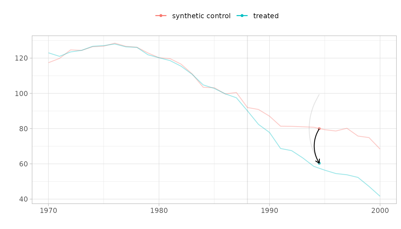

For DID, all control states receive equal weight and the counterfactual is a simple average. Notice that the pre-treatment fit is worse—DID does not optimize weights to match California’s trajectory:

plot(did_est, se.method = "placebo")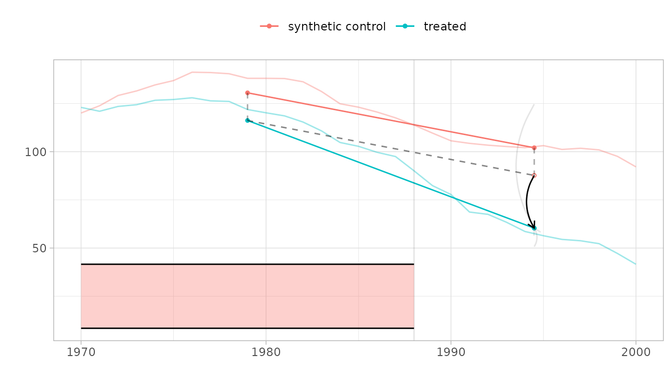

Comparing Weight Distributions

The difference between methods becomes concrete when you look at the weights they assign. SDID and SC concentrate weight on a few informative donors, while DID spreads it uniformly:

omega_comparison <- data.frame(
  unit = seq_along(attr(sdid_est, "weights")$omega),
  SDID = attr(sdid_est, "weights")$omega,
  SC   = attr(sc_est, "weights")$omega,
  DID  = attr(did_est, "weights")$omega
) |>
  tidyr::pivot_longer(-unit, names_to = "method", values_to = "weight") |>
  dplyr::filter(weight > 0.001)

ggplot(omega_comparison, aes(x = reorder(factor(unit), -weight), y = weight)) +
  geom_col(fill = "steelblue", alpha = 0.8) +
  facet_wrap(~ method, scales = "free_x") +
  labs(x = "Control Unit Index", y = "Weight (ω)",
       title = "Unit Weight Distributions by Method",
       subtitle = "Only nonzero weights shown") +
  theme_minimal(base_size = 10) +
  theme(axis.text.x = element_blank(), panel.grid.major.x = element_blank())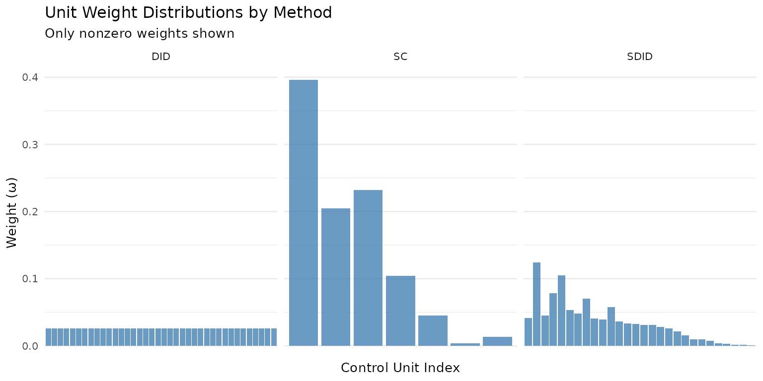

Predictions and Effect Curves

The predict() method provides three types of output:

Counterfactual: What Would Have Happened Without Treatment

# Counterfactual trajectory for California (what would have happened)
counterfactual <- predict(sdid_est, type = "counterfactual")
counterfactual[, (ncol(counterfactual) - 4):ncol(counterfactual)]
#>      1996      1997      1998      1999      2000 
#>  99.20256 100.03594 100.43399  98.49735  91.43730

Treated: What Actually Happened

# Observed outcomes for California
treated <- predict(sdid_est, type = "treated")
treated[, (ncol(treated) - 4):ncol(treated)]
#> 1996 1997 1998 1999 2000 
#> 54.5 53.8 52.3 47.2 41.6

Effect Curve: Period-by-Period Treatment Effects

The average treatment effect (coef()) summarizes the post-treatment period into a single number. But the effect may vary over time. The effect curve decomposes it into per-period effects:

effect <- predict(sdid_est, type = "effect")

plot(effect, type = "b", pch = 19,
     xlab = "Post-Treatment Year",
     ylab = "Treatment Effect (packs per capita)",
     main = "Effect of Prop 99 on Cigarette Consumption Over Time")
abline(h = coef(sdid_est), lty = 2, col = "steelblue")
abline(h = 0, col = "grey50")
legend("bottomleft",
       legend = c("Per-period effect", "Average effect"),
       lty = c(1, 2), col = c("black", "steelblue"), bty = "n")

The effect grows over time, suggesting that the cigarette tax had a compounding impact on smoking behavior.

Standard Errors and Inference

Computing Standard Errors

Pass se = TRUE to compute standard errors during estimation:

result_with_se <- synthdid(PacksPerCapita ~ treated,
                           data = california_prop99,
                           index = c("State", "Year"),
                           se = TRUE,
                           se_method = "placebo")

# Standard error is stored as an attribute
attr(result_with_se, "se")
#> [1] 9.493824

Available SE Methods

Three standard error methods are available:

Method	Best for	Speed
`bootstrap`	Multiple treated units	Slow
`jackknife`	Quick diagnostics	Moderate
`placebo`	Single treated unit, many controls	Slow

Placebo re-estimates the treatment effect using each control unit as if it were treated. The SE is the standard deviation of these placebo estimates. This is the recommended method when there is a single treated unit and many controls.

Bootstrap resamples control units with replacement. It works best with multiple treated units.

Jackknife leaves out one control unit at a time. It is the fastest method but may underestimate uncertainty.

Confidence Intervals

confint(result_with_se, level = 0.95)
#>             Lower    Upper
#> treated -34.21134 3.003767

Parallel Processing

Bootstrap and placebo SEs are embarrassingly parallel—each replication is independent. You can speed them up with the future package:

library(future)
plan(multisession, workers = 4)

result <- synthdid(PacksPerCapita ~ treated,
                   data = california_prop99,
                   index = c("State", "Year"),
                   se = TRUE, se_method = "placebo")

plan(sequential)  # Reset when done

Built-In Plotting

Trajectory Plot

# Default plot: treated vs synthetic control with effect diagram
plot(result_with_se)

Overlaying Trajectories

When trajectories are far apart, it can be hard to assess parallel trends. Use overlay to shift the control toward the treated unit:

# Overlay = 1 aligns pre-treatment levels
plot(result_with_se, overlay = 1)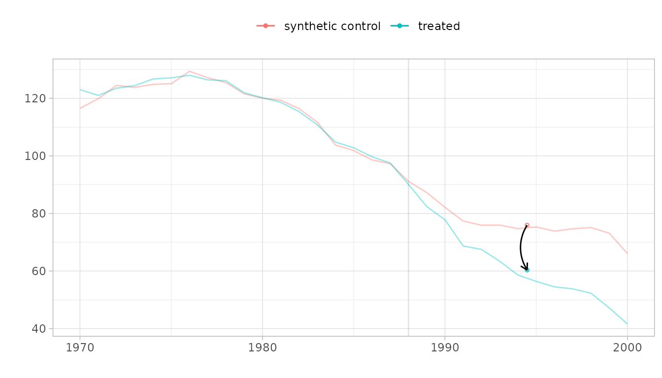

Unit Contributions

The synthdid_units_plot() shows how each control unit contributes to the estimate. Dot size reflects the unit weight $\omega_i$ :

synthdid_units_plot(result_with_se)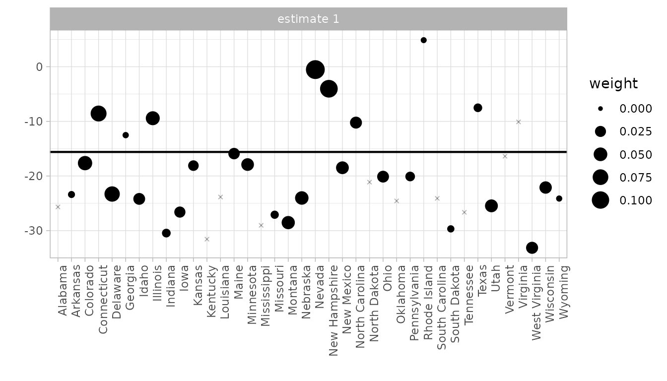

Multi-Estimator Comparison

Compare estimators side-by-side using synthdid_plot() with a named list:

estimates <- list(
  "Diff-in-Diff"  = did_est,
  "Synth Control"  = sc_est,
  "Synth DID"      = sdid_est
)
synthdid_plot(estimates, se.method = "placebo")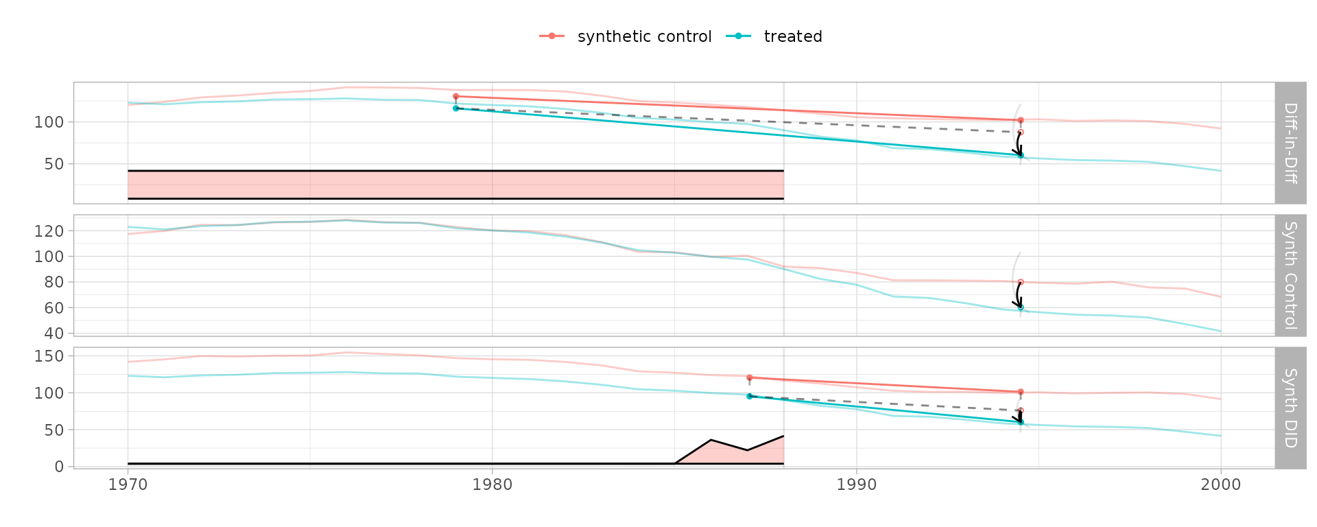

Convergence and Optimization Parameters

The SDID weights are estimated by a Frank-Wolfe (conditional gradient) optimization algorithm. Like all iterative algorithms, convergence is not guaranteed within a fixed number of iterations. The package monitors convergence automatically and warns you when it fails.

Checking Convergence

# Boolean: did the optimization converge?
synthdid_converged(result)
#> [1] FALSE

# Detailed diagnostics
synthdid_convergence_info(result)
#> Synthdid Convergence Diagnostics
#> =================================
#> 
#> Overall Status: NOT CONVERGED 
#> 
#> Lambda weights optimization:
#>  converged iterations max_iter utilization
#>      FALSE      10000    10000      100.0%
#> 
#> Omega weights optimization:
#>  converged iterations max_iter utilization
#>      FALSE      10000    10000      100.0%
#> 
#> Recommendation: Consider increasing max.iter or relaxing min.decrease threshold.

If synthdid_converged() returns FALSE, the estimate may be unreliable. The most common fix is to increase max.iter.

Optimization Parameters

The following parameters can be passed via ... to synthdid() to control the optimization. These are forwarded to synthdid_estimate():

Regularization

Parameter	Default	Description
`eta.omega`	$(N_1 \cdot T_1)^{1/4}$	Regularization strength for unit weights. Higher values shrink omega toward uniform weights.
`eta.lambda`	`1e-6` (near-zero)	Regularization strength for time weights. Kept small so lambda is data-driven.
`noise.level`	SD of first-differences of control outcomes	Scale factor that converts eta to zeta: `zeta = eta * noise.level`.

The regularization penalty in the Frank-Wolfe objective is $\zeta^2 \cdot \| \omega \|_2^2$ (and analogously for lambda). Larger eta.omega pulls the solution toward uniform weights, making SDID behave more like DID. Setting eta.omega to near-zero makes it behave more like SC.

# More regularization: pulls weights toward uniform (DID-like)
result_strong_reg <- synthdid(PacksPerCapita ~ treated,
                              data = california_prop99,
                              index = c("State", "Year"),
                              eta.omega = 10)
coef(result_strong_reg)
#>  treated 
#> -18.3726

# Less regularization: sparser weights (SC-like)
result_weak_reg <- synthdid(PacksPerCapita ~ treated,
                            data = california_prop99,
                            index = c("State", "Year"),
                            eta.omega = 0.01)
coef(result_weak_reg)
#>   treated 
#> -10.65604

Convergence Control

Parameter	Default	Description
`max.iter`	`10000`	Maximum Frank-Wolfe iterations. Increase if you see convergence warnings.
`min.decrease`	`1e-5 * noise.level`	Stop when the objective decrease per iteration falls below `min.decrease^2`. Smaller values demand tighter convergence.

# Tighter convergence: more iterations, stricter stopping
result_tight <- synthdid(PacksPerCapita ~ treated,
                         data = california_prop99,
                         index = c("State", "Year"),
                         max.iter = 50000,
                         min.decrease = 1e-8)
synthdid_converged(result_tight)
#> [1] FALSE

Intercepts

Parameter	Default	Description
`omega.intercept`	`TRUE`	Include an intercept when fitting unit weights. Allows the synthetic control to match trends rather than levels.
`lambda.intercept`	`TRUE`	Include an intercept when fitting time weights.

Disabling intercepts makes SDID behave more like SC (requiring level matching rather than trend matching):

result_no_intercept <- synthdid(PacksPerCapita ~ treated,
                                data = california_prop99,
                                index = c("State", "Year"),
                                omega.intercept = FALSE)
coef(result_no_intercept)
#>  treated 
#> -18.7527

Sparsification

Parameter	Default	Description
`sparsify`	Internal function	After an initial optimization, weights below `max(weight)/4` are set to zero and the optimization is re-run. Set to `NULL` to disable.
`max.iter.pre.sparsify`	`100`	Maximum iterations for the first (pre-sparsification) optimization round.

Sparsification produces cleaner, more interpretable weights at the cost of slightly less optimal fit. Disable it if you want the raw Frank-Wolfe solution:

result_no_sparse <- synthdid(PacksPerCapita ~ treated,
                             data = california_prop99,
                             index = c("State", "Year"),
                             sparsify = NULL)

# Compare number of nonzero weights
cat("With sparsification:",
    sum(attr(result, "weights")$omega > 1e-6), "nonzero donors\n")
#> With sparsification: 28 nonzero donors
cat("Without sparsification:",
    sum(attr(result_no_sparse, "weights")$omega > 1e-6), "nonzero donors\n")
#> Without sparsification: 38 nonzero donors

Pre-Specified Weights

You can supply your own weights instead of estimating them. By default, supplying a weight vector fixes it (it is not re-optimized). Use update.omega = TRUE or update.lambda = TRUE to use supplied weights as initialization for further optimization instead.

Parameter	Default	Description
`weights`	`list(omega = NULL, lambda = NULL)`	Pre-specified weight vectors. If non-NULL, used instead of optimizing.
`update.omega`	`FALSE` if `weights$omega` given	If `TRUE`, use supplied omega as initialization and re-optimize.
`update.lambda`	`FALSE` if `weights$lambda` given	If `TRUE`, use supplied lambda as initialization and re-optimize.

setup <- attr(result, "setup")

# Use uniform lambda (makes SDID behave like SC + intercept)
result_uniform_lambda <- synthdid(
  PacksPerCapita ~ treated,
  data = california_prop99,
  index = c("State", "Year"),
  weights = list(lambda = rep(1 / setup$T0, setup$T0), omega = NULL)
)
coef(result_uniform_lambda)
#>  treated 
#> -16.1212

Residuals and Diagnostics

The formula interface provides residual extraction for model diagnostics:

# Control-unit residuals (how well does the model fit control outcomes?)
resid_control <- residuals(result, type = "control")
cat("Control residuals: ", nrow(resid_control), "units x",
    ncol(resid_control), "periods\n")
#> Control residuals:  38 units x 31 periods
cat("Mean absolute residual:", round(mean(abs(resid_control)), 2), "\n")
#> Mean absolute residual: 22.72

# Pre-treatment residuals (quality of pre-treatment fit)
resid_pre <- residuals(result, type = "pretreatment")
cat("Pre-treatment RMSE:", round(sqrt(mean(resid_pre^2)), 2), "\n")
#> Pre-treatment RMSE: 21.99

Covariate Adjustment

If your data includes time-varying covariates, include them with the | operator in the formula:

# Syntax for covariate adjustment (requires covariates in your data)
result_cov <- synthdid(outcome ~ treatment | covariate1 + covariate2,
                       data = your_data,
                       index = c("unit", "time"))

The covariates are used to partial out their effect before estimating the treatment effect. Internally, a regression coefficient beta is estimated for each covariate and subtracted from the outcome matrix.

Summary

Quick Reference

Task	Code
Estimate SDID	`synthdid(y ~ w, data, index)`
Estimate SC	`synthdid(y ~ w, data, index, method = "sc")`
Estimate DID	`synthdid(y ~ w, data, index, method = "did")`
Point estimate	`coef(result)`
Confidence interval	`confint(result)`
Summary with SE	`summary(result)`
Effect curve	`predict(result, type = "effect")`
Counterfactual	`predict(result, type = "counterfactual")`
Treated trajectory	`predict(result, type = "treated")`
Residuals	`residuals(result, type = "control")`
Convergence check	`synthdid_converged(result)`
Plot	`plot(result)`
Unit contributions	`synthdid_units_plot(result)`
Switch method	`update(result, method = "did")`
Inspect weights	`attr(result, "weights")`

Next Steps

vignette("formula-interface") — deep dive on the formula interface
vignette("more-plotting") — plotting gallery with customization examples
vignette("convergence-diagnostics") — troubleshooting convergence
vignette("parallel-processing") — speeding up SE computation

References

Arkhangelsky, D., Athey, S., Hirshberg, D. A., Imbens, G. W., & Wager, S. (2021). Synthetic Difference in Differences. American Economic Review, 111(12), 4088–4118.