Parallel benchmarking for standard errors
Source:vignettes/benchmarking-parallel.Rmd
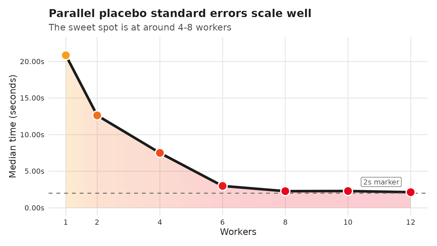
benchmarking-parallel.RmdThis vignette sketches how to benchmark the speedups from
parallelizing standard error computation in synthdid using
future/furrr. The benchmarks below vary the
number of workers across {1, 2, 4, 6, 8, 10} and record elapsed times.
Because exhaustive runs can be time-consuming, the benchmarking chunk is
not evaluated during vignette build; you can copy-paste and run it
locally.
Setup
We use the built-in California Proposition 99 example and compute
bootstrap standard errors, which are parallelized internally via
furrr.
Benchmark script (run locally)
if (!requireNamespace("bench", quietly = TRUE)) {
  stop("Install the 'bench' package to run these benchmarks.")
}
set.seed(12345)
bench_bootstrap <- function(workers, trials = 100) {
  old_plan <- future::plan()
  on.exit(future::plan(old_plan), add = TRUE)

  future::plan(future::multisession, workers = workers)

  bench::mark(
    se = sqrt(vcov(tau_hat,
                   method = "placebo")),
    iterations = trials,
    check = FALSE
  )
}

candidate_workers <- c(1, 2, 4, 6, 8, 10, 12)
max_workers <- future::availableCores()

results <- purrr::map_dfr(
  candidate_workers[candidate_workers <= max_workers],
  \(w) {
    res <- bench_bootstrap(w)
    transform(
      as.data.frame(res),
      workers = w
    )
  }
)
# results %>% as_tibble() %>% select(workers, min:total_time)
# # A tibble: 7 × 9
#   workers      min   median `itr/sec` mem_alloc `gc/sec` n_itr  n_gc total_time
#     <dbl> <bch:tm> <bch:tm>     <dbl> <bch:byt>    <dbl> <int> <dbl>   <bch:tm>
# 1       1   15.79s   20.85s    0.0491    2.13GB  0.596       8    97      2.71m
# 2       2   10.29s   12.63s    0.0797    1.42MB  0.00693    92     8     19.24m
# 3       4    5.53s    7.51s    0.135   811.62KB  0.0117     92     8     11.39m
# 4       6    2.43s    2.99s    0.284     1.05MB  0.0247     92     8       5.4m
# 5       8    1.97s    2.28s    0.439      1.3MB  0.0543     89    11      3.38m
# 6      10    2.04s     2.3s    0.434     1.56MB  0.0537     89    11      3.42m
# 7      12    1.92s    2.14s    0.468     1.81MB  0.0578     89    11      3.17m
results <- structure(
  list(
    workers = c(1, 2, 4, 6, 8, 10, 12),
    min = structure(c(15.789292630041,
10.2873354259646, 5.52902677597012, 2.43353319703601, 1.96598740702029,
2.03453747311141, 1.9237926058704), class = c("bench_time", "numeric"
)),
    median = structure(c(20.8516474730568, 12.6315311414655,
7.5070378840901, 2.99263541400433, 2.27918024314567, 2.29857611202169,
2.13922449899837), class = c("bench_time", "numeric")),
    `itr/sec` = c(0.0491432426685301,
0.0796970034344533, 0.134640868811313, 0.284005025515579, 0.439304938966377,
0.434186054343806, 0.467500846884824),
    mem_alloc = structure(c(2287274568,
1488824, 831104, 1099376, 1365216, 1633264, 1899904), class = c("bench_bytes",
"numeric")),
    `gc/sec` = c(0.595861817355928, 0.00693017421169159,
0.0117079016357664, 0.0246960891752678, 0.0542961160520241, 0.0536634449188973,
0.0577810035475626),
    n_itr = c(8L, 92L, 92L, 92L, 89L, 89L, 89L
),
    n_gc = c(97, 8, 8, 8, 11, 11, 11),
    total_time = structure(c(162.789420591551,
1154.37213490298, 683.29921525484, 323.937929735519, 202.592759847874,
204.981249650009, 190.373986684834), class = c("bench_time",
"numeric"))),
  row.names = c(NA, -7L),
  class = c("tbl_df", "tbl", "data.frame"))

results %>%
  ggplot(aes(workers, median)) +
  geom_area(aes(fill = median), alpha = 0.2, color = NA) +
  geom_line(color = "#1c1c1c", linewidth = 1.6) +
  geom_hline(yintercept = 2, linetype = "dashed", color = "#6f6f6f", linewidth = 0.6) +
  annotate("label", x = max(candidate_workers) - 0.3, y = 2, label = "2s marker",
           vjust = -0.7, hjust = 1, size = 3.3, label.size = 0, color = "#4a4a4a") +
  geom_point(aes(fill = median), size = 4.8, shape = 21,
             stroke = 1.2, color = "white") +
  scale_fill_gradientn(colors = c("#EB001B", "#F79E1B")) +
  scale_x_continuous(breaks = candidate_workers) +
  scale_y_continuous(
    labels = scales::label_number(accuracy = 0.01, suffix = "s"),
    expand = expansion(mult = c(0.05, 0.12))
  ) +
  guides(fill = "none") +
  labs(
    title = "Parallel placebo standard errors scale well",
    subtitle = "The sweet spot is at around 4-8 workers",
    x = "Workers",
    y = "Median time (seconds)"
  ) +
  theme_minimal(base_size = 12) +
  theme(
    plot.background = element_rect(fill = "white", color = NA),
    panel.background = element_rect(fill = "white", color = NA),
    panel.grid.major = element_line(color = "#e6e6e6"),
    panel.grid.minor = element_blank(),
    axis.text = element_text(color = "#1c1c1c"),
    axis.title = element_text(color = "#1c1c1c"),
    plot.title = element_text(color = "#1c1c1c", face = "bold"),
    plot.subtitle = element_text(color = "#4a4a4a"),
    plot.margin = margin(t = 12, r = 12, b = 12, l = 12)
  )
Notes
-
furrralready uses deterministic RNG streams when.options = furrr::furrr_options(seed = TRUE)is set (as insynthdid), so parallel runs remain reproducible given the same seed. -
future::multisessionmay be unavailable or limited on some systems (e.g., CRAN macOS/Windows builders). In that case,futurewill fall back to a sequential plan. - Adjust
replicationsandtrialsto balance runtime and precision when benchmarking on your hardware.
BLAS Threading Considerations
The synthdid package uses RcppArmadillo for optimized
linear algebra, which relies on your system’s BLAS (Basic Linear Algebra
Subprograms) library. Some BLAS implementations are multi-threaded,
which can conflict with future::multisession
parallelism.
Default BLAS by Platform
| Platform | Default BLAS | Multi-threaded? |
|---|---|---|
| macOS | Apple Accelerate | Yes |
| Windows | Reference BLAS | No |
| Linux | Usually reference BLAS | No (unless OpenBLAS installed) |
Avoiding Thread Oversubscription
When using future::multisession with multiple workers,
each worker runs independent synthdid_estimate calls. If
your BLAS is also multi-threaded, you may experience thread
oversubscription:
4 workers × 4 BLAS threads = 16 threads competing for 8 cores → slower!Recommendation: Disable BLAS threading when using multiple workers:
# Disable BLAS threading (run before future::plan)
Sys.setenv(

  OPENBLAS_NUM_THREADS = 1,    # Linux with OpenBLAS
  MKL_NUM_THREADS = 1,         # Intel MKL

  VECLIB_MAXIMUM_THREADS = 1,  # macOS Accelerate

  OMP_NUM_THREADS = 1          # General OpenMP
)

# Now set up parallel workers
future::plan(future::multisession, workers = 4)
When to Use Multi-threaded BLAS
Multi-threaded BLAS is beneficial when:
- Running a single
synthdid_estimatecall (nofutureparallelism) - Working with large datasets (N0, T0 > 1000)
For bootstrap/jackknife standard errors with many replications on moderate-sized data, worker parallelism (many single-threaded workers) typically outperforms BLAS parallelism (fewer workers with multi-threaded BLAS).